1 Department of Anatomy and Reproductive Biology, University of Hawai 'i School of Medicine, Honolulu, HI, 96822
2 Plastination Laboratory, Institute of Anatomy, Vienna University, Wahringerstrasse, 1313 A-1090,
Vienna, Austria
3 Department of Computer Science, University of Saskatchewan , Saskatoon, SK, S7N 5E5
Computerized reconstruction of anatomical structures is becoming very useful for developing anatomical teaching modules and animations. Although databases exist consisting of serial sections derived from frozen cadaveric material, plastination represents an alternate method for developing anatomical data useful for computerized reconstruction. The purpose of this study was to describe a method for developing a computerized model of the human kidney and ureter using plastinated tissue. A human kidney was obtained, plastinated , sectioned and subjected to 3D computerized reconstruction using the WinSURF modeling system (SURFdriver Software). The kidney was generated rapidly and rendered easily on a Windows laptop machine in real time. Qualitative observations revealed that the morphological features of the model were consistent with those displayed by typical cadaveric specimens. Morphometric analysis indicated that the model did not differ significantly from a sample of cadaveric specimens. These data support the use of plastinated tissue for generating tissue sections useful for 3D computerized modeling .
plastination; E12; kidney; computer; modeling; SURFdriver
S. Lozanoff, Telephone 808-956-8424 ; Fax 808-956-8491 ; email: Lozanoff@hawaii.edu

![]()


Gross Anatomy consumes a large portion of the first year of training in U.S. Medical Schools requiring approximately 150 hours of contact time (Drake et al.,2002). Human dissection continues to be seen as the primary means of learning human anatomy and this should be a priority for medical students (Aziz et al., 2002). However, new modalities are emerging as a means to supplement certain experiences not easily simulated with cadaveric material . For example, Project TOUCH (http://hsc.unm.edu/touch) is a collaborative effort between the University of Hawai 'i and the University of New Mexico medical schools aimed at developing problem based learning (PBL) cases that can be distributed via the National Computational Science Alliance' Access Grid (http://archive .ncsa.uiuc.edu/alliance/access-dc/) simultaneously across large distances (Jacobs et al., 2003). The objective of this project is to generate a virtual patient that can be treated simultaneously by students at remote locations within a PBL context (Caudell et al., 2003). Electronic anatomical models are becoming increasingly important as they can be transmitted across the internet within the case (Lozanoff et al., 2003).
Computer models and animations of anatomical features are becoming increasingly attractive as a means to communicate complex spatial relationships and concepts effectively (Dev et al., 2002). Although many educational animations are based on artistic renderings (Johnson and Whitaker, 1994; Habbal and Harris, 1995; Gould, 2001), more recent applications are using virtual representations derived from actual cadaveric material (Neider et al., 2000; Lozanoff et al., 2003). Within the medical curriculum, anatomical specimens can be used to develop animations and to incorporate into didactic lectures providing insight into function and spatial relationships not easily conveyed through static 2D images (Trelease et al. 2000; Neider et al., 2000). However, anatomical modeling traditionally has been difficult for the individual instructor due to the limited availability of low cost software that can be implemented on an individual desktop or laptop computer. Similarly, the quantity of cross sectional image data useful for three-dimensional modeling is limited .
The Visible Human Male (VHM) and Visible Human Female (VHF) datasets developed through the National Library of Medicine (NLM) provide a valuable resource of image data even to the individual instructor with only desktop computer modeling capabilities (Spitzer and Whitlock, 1998; Jastrow and Vollrath, 2003). Even though these data sets are extremely impressive and useful , representation has been a problem for some organs and tissues. For example, no attempt was made to infuse hollow organs to prevent their collapse and thus certain structures are difficult to reconstruct accurately.
The purpose of this paper is to present the use of serially sectioned plastinated tissues for generating anatomical reconstructions using a simple desktop modeling system. The kidney was selected as the subject for its potential use in simulated renal failure problem based learning cases within a medical school curriculum (Jacobs et al., 2003).
Tissue Processing
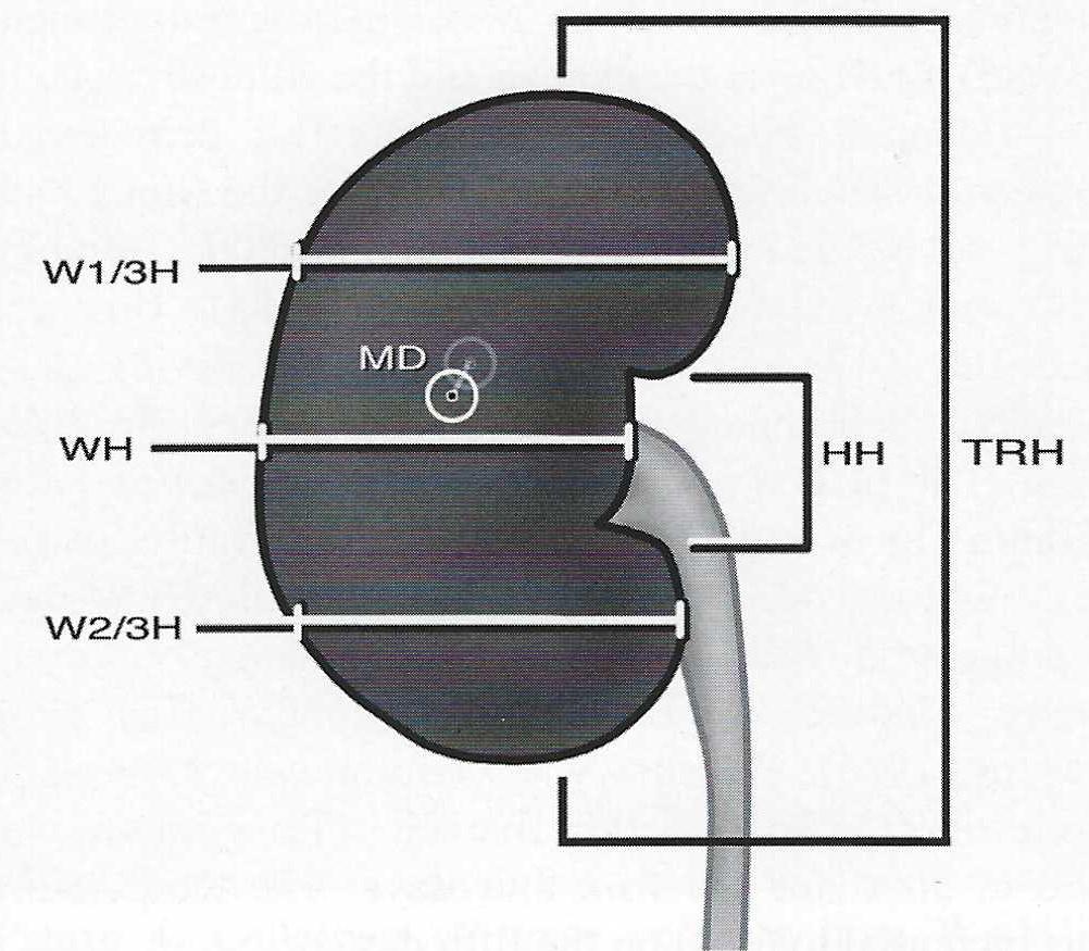
Figure l . Locations of measurements recorded from the kidney reconstruction and cadaveric specimens. TRH, total renal height; HH, hilum height; MD, maximum depth; WH, width at hilum; W l /3H, width at 1/3rd height of kidney; W2/3H, width at 2/3rds height of kidney.
One human kidney (right) was removed from a fresh unfixed cadaver (female, 80 years old with no apparent pathology), measured and finally plastinated as described by von Hagens (1985). Measurements taken were the length of the kidney from superior to inferior poles (TRH), width of the anterior surface of the kidney at the level of the hilus (WH), width of the anterior surface of the kidney at 1/3 and 2/3 of TRH (W l/3H and W2/3H) and height of the hi l us (HH) (Fig.1 ). Kidney thickness was measured at the point at which the kidney appeared thickest (MD) (Fig. 1). The needles which were used to indicate the initial measurement points were left in place to be used again following plastination for accurate re-measurement of the kidney for determination of tissue shrinkage. The kidney was kept frozen at -80°C for one week before being placed into a freezer at -25°C for 2 days. The 25 liters of technical quality acetone used for dehydration of the kidney was cooled to -25°C in a freezer. The acetone was divided into three aliquots to form three sequential dehydration baths. The kidney was allowed to dehydrate in the first acetone bath for four weeks. The lengths of the second and third dehydration baths were three and two weeks respectively. The concentration of the three acetone aliquots at the end of the three baths was measured to be 92%, 97% and 99% respectively (Table 1).
| Temperature | Days | |
| Fresh | -80°C/-25°C | 7/2 |
| AC1 | -25°C (96%) | 28 |
| AC2 | -25°C (97%) | 21 |
| AC3 | -25°C (99%) | 14 |
| MC1 | l15°C | 28 |
| Impregnation | 30°C/60°C | 411 |
| Curing | 65°C | 4 |
With dehydration complete, the freezer was disconnected and the specimen reached room temperature (15°C) after 24 hours. The acetone was changed with room temperature methylene-chloride (MeCl) for degreasing of the specimen. Degreasing was deemed sufficient when the MeCl bath appeared clear instead of yellow at the change and the adipose tissue in the specimen became transparent. The dehydrated, degreased specimen was removed from the MeCl bath and submerged in a El2/E6/A E600 mixture (100/50/0.2by volume) (von Hagens, 1985). This was placed in a Heraeus VT 6130 M vacuum drying oven (Haraeus Instruments, Kendra Laboratory Products GmbH) at 30°C. Pressure in the oven was decreased to 350mm Hg overnight to commence penetration of the El2 mixture into the specimen. The following day, impregnation was continued at 30°C using a second epoxy mixture of El2/E6/E600 (100/50/0.2) (von Hagens, 1985). Pressure was continuously reduced to the level of 2mm Hg within five days. Temperature was held at 30°C for the first four days. The temperature was increased to 60°C on the fifth day.
Once impregnation was complete, the specimen was removed from the vacuum and placed in a rectangular mold built of Styrofoam and lined internally with polyethylene foil. The mold containing the impregnated specimen and embedding medium was returned to the oven at 65°C for 4 days. After the block cooled to room temperature, the mold was carefully removed. The El2 block measured 150xl00xl00mm. The El2 block was serially sectioned using a diamond blade band saw (Exact 310 CP; Exact Apparatebau GmbH, Norderstedt, Germany). The average thickness of sections was 0.6mm. Due to the thickness of the saw blade, 0.4rnm of specimen was lost between sections. Each section was coated with polymer reaction mixture El2 :E l (100:28) (von Hagens, 1985; Weber and Henry, 1993) and cast between two layers of polyester foil. The foil plates containing the laminated slices were allowed to cure for 24 hours at room temperature after which they were placed in an oven at 45°C for 24 hours. This procedure provided the sections with a smooth, refinished polymer surface devoid of refractive artifacts caused by cutting with a saw.
To determine shrinkage resulting from the plastination process, the kidney was remeasured following plastination.
Computer Modeling
Laminated slices were scanned using an EPSON GT- 10000+ Color Image Scanner at 600 dpi. Placement of slices on the scanner bed occurred with the inferior surface of the laminate resting on the glass of the bed . A ruler (mm) was included with every scan as a calibration marker. Although the scanned images could have been used directly for computer modeling, we decided to include an extra step involving manual tracing so that alignment could by more closely controlled . Scanned images of the tissue slices were printed and manually traced. Alignment guides were transferred to each tracing. Each manual tracing was placed on a scanner so that fiducial points aligned with a base alignment tracing attached to the scanning bed . Once scanned, these images (jpeg format) were loaded into WinSURF (SURFdriver 4.0 ; http://www.surfdriver.com) and traced from the monitor . Features used in the reconstruction , defined as objects, included the kidney parenchyma (cortex and medulla) and ureter. Each object was traced and numbered accordingly. Once all contours were traced, the reconstruction was rendered and visualized and the model was qualitatively checked for surface discontinuities in the renal cortex, renal medulla and ureter by rotating the model and viewing. Kidney and ureter textures were applied using SURFdriver maps (www.surfdrivermaps .com). System execution times and data array features were recorded as an index of program efficiency.
Once rendered, the measuring tool available in WinSURF was used to record height, width and depth measurements from the model. Measurements , TRH, WH, W l/3H, W2/3H, HH, MD, were also recorded from 12 cadaveric specimens using a Helios Caliper (0.l mm). Average values and their standard deviations were also recorded for the cadaveric specimens. The corresponding measurements taken from the model were used and a weighted mean difference was calculated (t5) . Statistical significance was determined at the p < 0.05 level using a sample observation compared to a population mean test (Sokal and Rohlf, 1981:229- 231).
Prior to plastination, the length of the kidney from the superior pole to the inferior pole was 10.2lcm while the width in the middle of the anterior surface was 4.72cm. Following plastination , the length of the kidney measured 10. 16cm while the width was measured to be 4.69cm. Hence, the amount of overall shrinkage of the specimen was calculated to be 5.23%.
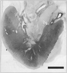 Figure 2. A representative section of the plastinated kidney. Scale = 1 .5 cm. |
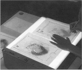 Figure 3. Manual tracing of plastinated specimens |
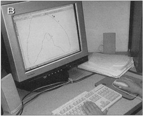 Figure 4. Collection of tissue contours from WinSURF generated images of scanned specimen tracings. |
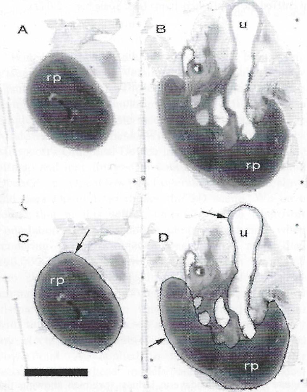 Figure 5. Representative tissue sections from superior (A) and middle (B) regions of the kidney. Tissue contours were traced (arrows in C,D) for the ureter and its branches (u) and renal parenchyma (cortex and medulla, rp) for all sections. These contours provided the data for the model. Scale bar = 2.0 cm . |
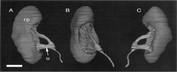 Figure 6. Rendered kidney viewed from the anterior (A), medial (B) and posterior aspects (C). Perirenal adipose tissue was not included in the model thus revealing the ureter (u) as it entered the renal parenchyma (rp). Scale bar = 2.0 cm |
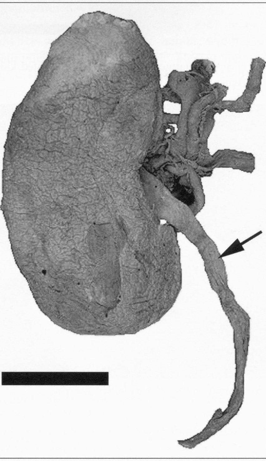 Figure 7. Typical cadaveric kidney specimen showing the ureter (u). Scale bar = 3.0 cm . |
Figure 2 shows the transparency and color of the laminated slices. The renal parenchyma was easily identified and the borders could be easily copied onto tracing paper (Fig. 3). Following this manual procedure , the traced contours were scanned and loaded into WinSURF and automatic edge detection was used to quickly collect tissue borders or contours (Fig. 4). These contours were visualized on the tissue borders and showed close continuity with the edges of the objects (Fig. 5). The rendered kidney showed a distinct parenchyma with calyces emptying into the ureter (Fig. 6). Renal fat was not reconstructed so the hilar region was clearly visible from the medial aspect. The kidney model was rendered and rotated in real time and i t compared well with a representative cadaveric kidney using qualitative observations (Fig. 7).
The digitally rendered kidney consisted of 9992 triangles on 4952 vertices while the ureter comprised 3553 triangles on 1730 vertices (Fig. 6). Triangulating the surface from the contours took 4.5 seconds on a 1 .5 GhZ machine with 5 l 2Mb RAM and an ATI Rad eon Graphics card. Rendering of the surfaced objects using OpenGL was virtually instantaneous, with or without the graphics card enabled. Thus, the model was moved smoothly in real time with the mouse pointer.
Quantitative measurements showed that the overall morphology was retained (Table 2). Weighted difference of the means and observed values differed very slightly with the greatest difference recorded for hilum height (HH, 1.68) and the smallest for maximum depth (MD, -0. 13). Coefficients of variation for the six variables ranged from a low of 11.3% to 19.5%. None of the variables recorded from the model were significantly different from the corresponding values measured from cadaveric specimens at the p < .05 level.
| Specimen Number | THR | HH | WH | MD | Wl/3H | W2/3H |
| 1 | 10.72 | 2.68 | 4.06 | 4.25 | 5.03 | 3.46 |
| 2 | 10.08 | 3.05 | 4.53 | 5.52 | 6.06 | 4.04 |
| 3 | 7.79 | 3.54 | 3.62 | 3.61 | 4.03 | 3.67 |
| 4 | 7.64 | 3.98 | 4.14 | 3.53 | 4.74 | 3.00 |
| 5 | 10.50 | 3.96 | 4.50 | 4.80 | 4.50 | 4.37 |
| 6 | 10.24 | 3.49 | 5.00 | 4.90 | 4.67 | 4.86 |
| 7 | 8.43 | 2.36 | 4.10 | 4.22 | 4.80 | 3.88 |
| 8 | 9.41 | 4.10 | 4. 16 | 3.50 | 3.76 | 4.22 |
| 9 | 9.83 | 4.63 | 5.00 | 5.36 | 5.45 | 4.16 |
| 10 | 10.82 | 4.50 | 5.49 | 4.88 | 4.77 | 4.90 |
| 11 | 10.07 | 3.05 | 4.44 | 4.58 | 4.72 | 4.29 |
| 12 | 9.51 | 3.64 | 4.29 | 4.03 | 4.26 | 4.84 |
| Mean (st dev) | 9.59 (1.09) | 3.58 (0.70) | 4.44 (0.51) | 4 .43 (0.69) | 4 .73 (0.61) | 4.14 (0.58) |
| Model Value | 9.42 | 4.81 | 4.25 | 4.34 | 4 .31 | 3.30 |
| ts | -0. 15 | l.68 | -0.37 | -0.13 | -0.67 | -1.39 |
| sig. level | ns | ns | ns | ns | ns | ns |
The system described here relies on relatively inexpensive hardware including a EPSON GT-10000+ scanner and Dell Laptop computer. The WinSURF reconstruction package from SURFdriver Softwere © (surface reconstruction driver), was developed expressly for use in three-dimensional anatomical reconstruction and it is a simple icon-driven system (Moody and Lozanoff, 1998). It has been shown to provide accurate and precise computer generated anatomical models (Lozanoff, 1992; 1999). Minimum requirements for the software are extremely modest and include a 200 MHz Intel Pentium processor, Windows 2000, Windows XP, Windows NT, 24 MB of free available systems RAM (64 MB recommended) , 50 MB of available disk space, 1024 x 768, 16-bit color display, CD ROM drive and 3 1/2" floppy or 100 MB Zip Drive, and a Microsoft Mouse or compatible pointing device; all of which comes with standard IBM equipment.
WinSURF reconstruction software was built using Visual Studio C++ Version 6.0, and subsequently Visual Studio .NET. The code was originally written using Microsoft Foundation Classes (MFC) with a Single Document Interface (SDI) to manage the windowing environment. Within MFC , WinSurf uses Microsoft's Graphical Device Interface (GDI) to display bitmap and jpeg images for contour tracing rather than OpenGL, as OpenGL's pixel operations were too slow, and uses OpenGL to render the 3D scene. We have found that in this setting OpenGL within Microsoft Foundation Classes exhibits choppy rendering when rendering OpenGL objects consisting of more than 200,000 triangles . As well, the output can be loaded into shareware available from the web that permits animation of complex movements . Thus, the individual instructor can develop very sophisticated animation with little effort and these can be incorporated directly into electronic presentations utilizing such programs as PowerPoint. As applied to the kidney and ureter reconstruction , these models are relatively modest objects computationally since they comprised 9992 triangles and were easily handled by the system for real time manipulation and display .
The kidney model generated displays a morphology that corresponds qualitatively to the actual cadaveric specimen . Perirenal fat was not reconstructed so that the hilus would be easily seen from the medical aspect of the model. This adipose probably could be reconstructed in subsequent experiments to achieve a realistic appearance for the model. Similarly, the ureter and major and minor renal calyces apparently collapsed and could be depicted more effectively if the collecting duct system had been dilated prior to plastination. Quantitative analysis of the model was based on a comparison of the reconstruction to a sample of cadaveric specimens. The coefficients of variation for each cadaveric specimen variable were relatively large (ranged from 11.3% to 19.5%) which probably contributed to the lack of significance. A larger cadaveric sample would probably provide a greater measure of accuracy for the model. Nonetheless , the model shows close morphometric correspondence to the cadaveric specimens with all variables not significantly different from the actual kidneys. Results generated from this analysis demonstrate that plastinated material can be used effectively to generate tissue contours suitable for computerized three-dimensional reconstruction.
A logical advantage of models is that they provide a greater sense of realism for the student and thus should permit the student to learn more information while reducing the time required. One could hypothesize tat this realism stimulates students to generate learning issues more effectively and possibly with a greater sense of urgency (Jacobs et al., 2003; Caudell et al., 2003). This effect remains largely untested and exists as a ripe area for educational investigation .
A major problem with existing anatomical databases is the low resolution for smaller anatomical structures. Large features are easily visible and can be modeled successfully for anatomical animations. However, many of the smaller structures such as arteries and nerves are not easily visible. Plastination provides a useful alternative for generating anatomical databases (Lozanoff et al., 2003, Qiu et al., 2003). These preserved tissues are significantly easier to cut, stain, and handle compared to fresh frozen tissue since they are much more durable owing to the silicon infiltrate. Plastinated tissues may provide much greater resolution compared to fresh frozen tissue sectioning, yet this remains to be tested. Although the scanned plastinated images could have been traced directly within the WinSURF editing window, it was decided to include an extra step involving manual tracing so that alignment could be more closely controlled. This step increased the processing time, but decreased postprocessing . Nonetheless, plastinating specimens locally enables anatomical computer models to be generated achieving very specific educational course objectives. Future work will be directed at developing datasets utilizing plastinated tissue and determining their usefulness for 3D reconstruction .
Acknowledgements: This presentation was made possible by NIH Grant Number RR-16467 from the BRIN Program of the National Center for Research Resources (SL). Beth K. Lozanoff provided the illustration in figure 1.
Aziz MA, McKenzie JC, Wilson JS, Cowie RJ, Ayeni SA Dunn BK. 2002 : The human cadaver in the age of 'biomedical informatics. Anat Rec (New Anat) 269 :20-32.
https://doi.org/10.1002/ar.10046
Caudell TP, Summers K, Holten J, Hakamata T, Mowafi M, Jacobs J, Lozanoff BK, Lozanoff S, Wilks D, Keep, MF, Saiki S, Alverson D. 2003: Virtual patient simulator for distributed collaborative medical education. Anat Rec, 270B:23-29.
https://doi.org/10.1002/ar.b.10007
Dev P Montgomery K, Senger S, Heinrichs WL, Srivastava S, Waldron K. 2002 : Simulated medical learning environments on the internet. J Amer Med Informatics Assoc 9:437-447.
https://doi.org/10.1197/jamia.M1089
Drake RL, Lowrie DJ, Prewitt CM. 2002 : Survey of gross anatomy, microscopic anatomy, neuroscience, and embryology courses in medical school curricula in the United States. Anat Rec (New Anat) 269 : 118- 122.
https://doi.org/10.1002/ar.10079
Gould DJ. 2001: The brachia} plexus: Developmental and assessment of a computer based learning tool. Med Educ Online 6: 1-7.
https://doi.org/10.3402/meo.v6i.4525
Habbal OA, Harris PF. 1995: Teaching of human anatomy: a role for computer animation. J Audiovisual Media Med 18:69-73.
https://doi.org/10.3109/17453059509022997
Jacobs J, Caudell T, Wilks D, Keep MF, Mitchell S, Buchanan H, Saland L, Rosenheimer J, Lozanoff BK, Lozanoff S, Saiki S, Alverson D. 2003: Integration of advanced technologies to enhance problem-based learning over distance: Project TOUCH. Anat Rec 270B: 16-22.
https://doi.org/10.1002/ar.b.10003
Jastrow H, Vollrath L. 2003: Teaching and learning gross anatomy using modern electronic media based on the Visible Human Project. Clin Anat 16:44-54.
https://doi.org/10.1002/ca.10062
Johnson D, Whitaker R. 1995: A graphic, three dimensional teaching model to demonstrate the topography of the human heart. Clin Anat 8:407-411.
https://doi.org/10.1002/ca.980080607
Lozanoff S. 1992: Accuracy and precision of computerized models of the anterior cranial base in young mice . Anat Rec 134:618-624.
https://doi.org/10.1002/ar.1092340417
Lozanoff, S. 1999: Sphenoethmoidal growth, malgrowth and midfacial profile. In: On Growth and Form: Spatio-temporal Patterning in Biology. Chapter 19. MAJ Chaplain , Dr. GD Singh and Dr. J. McLachlan (eds.). John Wiley and Sons, p 357-372.
Lozanoff S, Lozanoff BK, Sora M-C, Rosenheimer J, Keep MF, Saland L, Tregear J, Jacobs J, Saiki .s' Alverson D. 2003: Anatomy and the access grid: exploiting plastinated brain sections for use in distributed medical education. Anat Rec 270B:30-37.
https://doi.org/10.1002/ar.b.10006
Moody D, Lozanoff S. 1998: SURFdriver: A practical computer program for generating three-dimensional models of anatomical structures using a PowerMac . Clin Anat 11:133.
Neider GL, Scott JN, Anderson MD. 2000 : Using QuickTime virtual reality objects in computer assisted instruction of gross anatomy : Yorick - the VR Skull. Clin Anat 13:287-293.
https://doi.org/10.1002/1098-2353(2000)13:4<287::AID-CA9>3.0.CO;2-L
Qiu M-G, Zhang S-X, Liu Z-J, Tan, L-W, Wang Y-S, Deng J-H, Tang Z-S. 2003: Plastination and computerized 3D reconstruction of the temporal bone. Clin Anat 16:300-303.
https://doi.org/10.1002/ca.10076
Spitzer VM, Whitlock DG. 1998. The Visible Human dataset: The anatomical platform for human simulation. Anat Rec (New Anat) 235:49-57.
https://doi.org/10.1002/(SICI)1097-0185(199804)253:2<49::AID-AR8>3.0.CO;2-9
Trelease RB, Nieder G, Dorup J, Hansen Schacht M. 2000: Going virtual with QuickTime VR: new methods and standardized tools for interactive dynamic visualization of anatomical structures. Anat Rec (New Anat) 261:64-77. https://doi.org/10.1002/(SICI)1097-0185(20000415)261:2<64::AID-AR6>3.0.CO;2-O
Trelease RB. 2002: Anatomical informatics : Millennial perspectives on a newer frontier. Anat Rec (New Anat) 269:224-235.
https://doi.org/10.1002/ar.10177
von Hagens G. 1985: Heidelberg plastination folder: Collection of technical leaflets for plastination. Anatomisches lnstitut 1, Universitiit Heidelberg, Heidelberg, p 1-14.
Weber W, Henry RW. 1993. Sheet plastination of body slices - El2 technique , filling method . J Int Soc Plastination 7(1): 16-22.
https://doi.org/10.56507/EZGX2343